Spreadsheets are supposed to save time, but sometimes they just make things messier. I hated digging through endless menus until I found a handful of formulas that do the heavy lifting for me.
VLOOKUP searches for a specific value in the first column of a range and returns a corresponding value from another column in the same row. You can call it a lookup tool that saves you from manually scrolling through vast datasets. The syntax for VLOOKUP is:

Here,search_keyis the value you want to find, andrangeis the table where you’re searching. Theindexparameter tells VLOOKUP which column to return data from, whileis_sortedindicates whether your data is sorted.
If you setis_sortedto FALSE, it will show you exact matches, which is usually what you want for most lookup tasks.
Here’s how VLOOKUP works in practice:
This formula searches for “Saniya” in column B and returns the corresponding value from the ninth column. It’s perfect if you want to find employee details, product information, or any data organized in tables.
However, there’s a limitation of VLOOKUP that it only searches to the right. It can’t look left of your search column. But for most everyday tasks, it handles data lookup perfectly. For more detailed examples, you may check out our guide onusing the VLOOKUP function in Google Sheets.

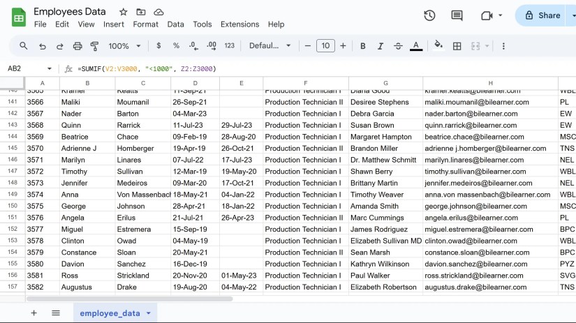
SUMIF adds up values in a range based on specific criteria you set. Instead of manually calculating totals for different categories, this formula does the heavy lifting, and it’s accurate.
While the basic IF function returns TRUE or FALSE based on conditions, SUMIF takes it further by performing calculations on the data that meets your criteria. It has the following syntax:

Here, therangecontains the cells you’re checking against your criteria, thecriteriais your condition, andsum_rangeis the actual values to add up. If you omit sum_range, SUMIF adds the values in the range itself. It only works with text, numbers, and even wildcards, such as asterisks (*) for partial matches.
In the above example, the formula checks column V for values less than 1000 and then sums the corresponding amounts in column Z. This formula is handy for calculating sales totals, expense categories, or any conditional summation.

How to Use the SUMIFS Function in Excel
Want to make data analysis in Excel a breeze? Learn how to use the SUMIFS function to quickly sum up specific criteria in your spreadsheets.
You can even combine multiple criteria, though you’ll need SUMIFS for that level of complexity. For such complex examples and advanced criteria combinations, you can check out our detailed guide onusing the SUMIF function in Google Sheets.
6CONCATENATE
This function combines text from multiple cells into a single cell. When you need to merge first and last names, create email addresses, or build custom labels, you can use this function in your formula to handle the text manipulation.
You can also use the ampersand (&) symbol as a shortcut for basic concatenation, thoughusing the CONCATENATE function in Google Sheetsoffers more flexibility for complex combinations. The syntax for CONCATENATE is:
Here,string1is your first text value, and you can add unlimited additional strings. Each parameter can be a cell reference, actual text in quotes, or a mix of both.
Remember that it doesn’t automatically add spaces, so you need to include them manually as separate parameters, as shown in the following example.
This formula combines the values from cells B2 and C2, separated by a space. It is perfect for creating full names, product codes, formatted addresses, and more.
CONCATENATE can become unwieldy if you use many parameters, but it’s still the most reliable way to merge text data. You can alsouse CONCATENATE in Excelto join text from multiple cells.
COUNTIF counts cells that meet specific criteria within a range. When you need to track how many items fall into certain categories—like counting completed tasks or tallying specific responses—this formula eliminates manual counting errors.
It works well for analyzing survey data, inventory tracking, and performance metrics. The syntax for COUNTIF is:
Here,rangespecifies the cells you want to examine, andcriteriadefine the condition that cells must meet to be counted. The criteria can include text, numbers, or logical operators. The following is an example:
This formula counts the number of cells in the range K2:K3000 that contain exactly the text “Active.” You canuse the COUNTIF function in Google Sheetsto track project statuses, count specific product types, or analyze categorical data.
COUNTIF also supports wildcards like asterisks (*) for partial text matches and question marks (?) for single-character substitutions.
you may also use comparison operators like “>50” or “>=100” to count numerical ranges. The formula is handy when dealing with large datasets where manual counting simply isn’t practical.
4ARRAYFORMULA
Next on the list is ARRAYFORMULA, which applies a single formula to an entire range of cells automatically. Instead of copying formulas down hundreds of rows, you write it once and let Google Sheets handle the rest.
I’ve found this useful when working with large datasets that constantly expand. Rather than remembering to drag formulas down every time new data appears, ARRAYFORMULA automatically keeps everything up to date. The basic syntax wraps your regular formula:
However, you need to reference entire columns or ranges rather than single cells. For instance, instead of A2, you’d use A2:A to include the whole column from row 2 downward.
Here’s a practical example that combines first and last names:
This formula concatenates every corresponding pair in columns B and C simultaneously. The results appear instantly across all rows with data. Moreover, it automatically adjusts when new rows are added.
For more examples, you can check out our guide on theARRAYFORMULA function in Google Sheets. It’s definitely worth the learning curve, especially if you work with data on a regular basis.
It extracts specific rows from a dataset based on the conditions you define. When you need to see only certain employees, projects, or sales records without manually hiding rows, this formula creates a dynamic subset instantly.
What I appreciate most about FILTER is that the results update automatically when your source data changes, unlike manual filtering. It is useful for live dashboards and reports. The syntax follows this pattern:
Therangecontains your data, whilecondition1specifies your first criterion. Additionally, you’re able to stack multiple conditions for more precise filtering, as shown in the example below.
This formula shows only Engineering department employees from the employee database. Consequently, you get exactly the subset you need without scrolling through irrelevant records.
FILTER works exceptionally well for project tracking, expense analysis, and client management, as it handles text and numerical criteria equally well.
If you want to see more detailed examples and filtering techniques, check out our guide on theFILTER function in Google Sheets. Honestly, it’s one of those formulas that genuinely saves hours of manual work when you’re constantly pulling different data subsets for reports and meetings.
QUERY brings database-style searching to Google Sheets using SQL-like language. While it might sound intimidating initially,this Google Sheets function can save you hours every week. It’s straightforward once you understand the basics and powerful for office data analysis.
It combines filtering, sorting, and grouping into a single formula. Instead of using multiple functions, you can extract exactly what you need with a single command. The basic syntax looks like this:
Thedataparameter contains your range, thequeryholds your SQL-like command in quotes, and theheadersspecify how many header rows to include. In the following example, QUERY analyzes employee performance data:
This formula retrieves employee names (column D), departments (column Q), and performance scores (column AB), then sorts by performance score in descending order. Essentially, you’re creating custom reports that otherwise would require you touse pivot tables in Excelor Google Sheets.
QUERY can be helpful in sales analysis, project tracking, and budget reporting as it handles text searches, date ranges, and mathematical operations. For more examples, you’re able to check out our detailed guide on theQUERY function in Google Sheets.
1IMPORTRANGE
This function directly imports data from other Google Sheets files into your current spreadsheet. When you’re managing multiple project files, budget trackers, or departmental reports, IMPORTNAGE can eliminate the copy-paste routine for you.
It maintains live connections between files. As a result, when your colleague updates the master sales spreadsheet, your dashboard automatically reflects those changes, and no manual updates are required. The syntax requires two key pieces of information.
Thespreadsheet_urlis the complete web address of the source file, while therangespecifies exactly which cells to import using standard notation, such as “Sheet1!A1:C10”. The following is an example:
This formula imports employee data from another department’s file directly into your consolidated report. But you’ll need to grant permission the first time, as Google Sheets will prompt you to connect the files.
IMPORTRANGE is handy for creating executive dashboards, consolidating team reports, and maintaining centralized data views, as it is theeasiest way to import data from another Google Sheets file. However, remember that too many IMPORTRANGE formulas can slow down your spreadsheet.
5 Ways to Import Data From a Website Into Google Sheets
Tired of copying and pasting data from websites? Learn how to import it directly into Google Sheets.
These eight formulas make spreadsheet work considerably easier. There is a learning curve involved, but the time savings become obvious once you’re using them regularly. Data tasks that used to take time will now happen in minutes, and that’s worth the effort.
